
What's My Transimpedance Q and f3db Bandwidth?
Sept 08, 2012
 The complex transimpedance transfer function Tz(f) of the circuit shown to the right is:

where Zf is the parallel impedance of Cf and Rf, Ao(f) is the op-amp open loop gain function and β(f) is the complex feedback fraction.
What is the 3db transimpedance bandwidth f3db and Q (Quality Factor) of this circuit? Since the circuit with the elements shown is a second order low-pass
filter identical in characteristics to the classic LRC passive filter, it is well known that the circuit exhibits resonant behaviour which can be described by a natural
undamped resonant frequency F0, a Quality factor Q which describes the "sharpness" of the resonance and a 3db response bandwidth f3db. Of course since the transimpedance
circuit is an active filter circuit, the actual values of F0, Q and f3db will depend in detail on the circuit parameters, GBW, Rf, Cf, Ri and Ci.
F0, Q and f3db can be written explicitly in terms of GBW and the circuit component values
but it is useful to write them in terms of the noise-gain zero and pole frequencies, Fz and Fp,
and the basic bandwidth BW and the DC noise gain N0:
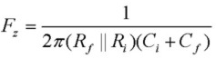

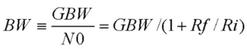
Note that for Ri>>Rf as is often the case for transimpedance amplifiers, N0 --> 1.0 and BW --> GBW.
In terms of these quantities, the natural undamped resonant frequency F0 of this transimpedance circuit is:

The Q value is given by:

and the 3db transimpedance bandwidth, in terms of F0 and Q, is given by:
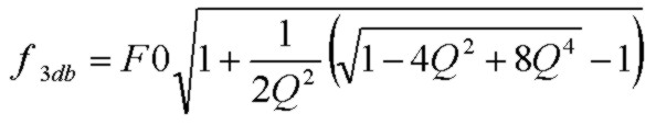
These expressions apply for any values of Ri, Ci, Rf and Cf and GBW with the assumption that the op-amp is ideal except for a finite GBW described
by a single-pole open-loop gain characteristic. Good transimpedance amplifier designs usually target
a Q in the range of 0.5 to 1.0
which provides good stability with adequate phase margin. A universal plot of Tz(f) is shown below for a wide range of Q values demonstrating how the transimpedance
response shape changes with damping.
The calculator below computes the f3db, Q, F0, Fz and Fp for the transimpedance circuit shown above. Enter the GBW, Rf, Ri, Cf, Ci values (note the units)
and click Get Params. Three convenient synthesis buttons are provided which determine the required value of Cf exactly for the three special cases of Q (if that value of Q is possible), given the GBW, Rf, Ri and Ci values.
A more comprehensive calculator is provided which also computes transimpedance circuit noise properties.
Isn't the transimpedance f3db bandwidth just the pole frequency Fp?
If the transimpedance response was determined solely by the pole due to Rf and Cf, then the f3db bandwidth would be equal to Fp. This would be
true for an ideal op-amp with infinite GBW product. It is fairly easy to show how the expression above for f3db in the general case reduces to Fp in that limit.
However, most design cases of interest which effectively utilize the available bandwidth of the op-amp with
values of Cf chosen for stability (i.e. with Q values of 0.5 to 1.0)
exhibit strong 2nd order response behaviour with peaking or flattening in the frequency response.
This modifies the f3db transimpedance bandwidth as reflected in the formula above.
How different is f3db from Fp? For the common case where Fp << GBW and Ri>>Rf, rewriting F0 and f3db in terms of Q and Fp, we have:

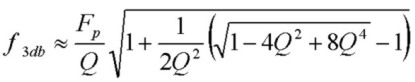
Then, with Cf chosen to produce these typical Q values and for cases where Cf << Ci, we find that the f3db bandwidth is considerably higher than Fp:
- Q=0.500 (critically damped case) f3db = 0.644F0 ~ 1.29Fp
- Q=0.707 (maximally flat case) f3db = 1.000F0 ~ 1.414Fp
- Q=1.000 ("PM=45 deg" case) f3db = 1.272F0 ~ 1.27Fp
Actual values will tend to be somewhat smaller than these ratios due to the finite value of Cf.
For example, consider an op-amp with a 200 MHz GBW and with Rf = 10kohm and Ci = 25pF. For the maximally flat Q=0.707 design, using the exact calculator above,
we need Cf = 1.99 pF creating a pole at Fp = 7.99 MHz resulting in a transimpedance bandwidth of f3db = F0 = 10.9 MHz, a ratio of 1.36.
A set of design charts for the Q=0.707 case is available for a wide range of Ci, Rf and GBW values.
See also the Wideband, High Sensitivity, Transimpedance Design example of the
OPA656 FET-input OPAMP Data Sheet.
Universal Transimpedance Curves
It is easy to show that the magnitude of the normalized (to DC transimpedance) complex transimpedance function |Tz(f)/Tz(0)|^2 is given by:

where x is the normalized frequency f/F0 and F0 is the natural resonant frequency given above.
The chart below shows a set of universal curves for values of Q from 0.1 to 3.0 in steps of 0.1.
The expressions given above relate F0 and Q to the actual circuit component values GBW, Rf, Cf, Ri, Ci.
The -3db line is shown. For transimpedance amplifiers, the most useful range for Q is between
0.5 and 1.0 as shown with black lines with the Q=0.7 line (close to the maximally flat response value of Q=1/√2) shown in green.
For the maximally flat case of Q=1/√2, x3db = 1.0 or f3db = F0 exactly.
The critically damped case with Q=0.50 corresponds to two independent cascaded single-pole low-pass filters with the same pole (cutoff) frequency of F0 resulting in f3db = 0.644F0.

Alternatively, the universal curves below show the normalized transimpedance as a function of the normalized frequency f/f3db where f3db is the -3db transimpedance bandwidth as given above
in terms of F0 and Q:

References