
The Perfect Transformer: Coupled Inductor Model
Mar 02, 2016
 The transformer is an inductive coupled device, intended to transform voltage and impedance levels in different parts of a circuit.
Real transformers (F. Langford-Smith 1957) include non-ideal effects such as wiring series resistance, shunt capacitances in the windings, iron-core losses etc.
This article summarizes the simplified perfect transformer model which is a coupled inductor model. This model must simplify to the most
basic and familiar ideal transformer model under certain limits as discussed below.
The transformer is an inductive coupled device, intended to transform voltage and impedance levels in different parts of a circuit.
Real transformers (F. Langford-Smith 1957) include non-ideal effects such as wiring series resistance, shunt capacitances in the windings, iron-core losses etc.
This article summarizes the simplified perfect transformer model which is a coupled inductor model. This model must simplify to the most
basic and familiar ideal transformer model under certain limits as discussed below.
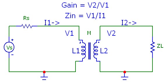
The perfect transformer model includes discrete inductors
representing the primary transformer winding with inductance L1, the secondary winding with inductance L2 and a mutual inductance M describing the magnetic-field inductive coupling between
the primary and secondary inductors. Basic theory shows that the maximum possible value for M is Sqrt(L1*L2) and any imperfect coupling is characterized
by a coupling constant k, where 0<k<=1. This model provides a useful, if not oversimplified model of the transformer. It enables very approximate
calculations of primary-to-secondary voltage gain and effective input impedance with arbitrary output load impedances.
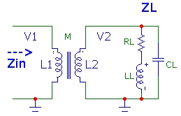
The diagram below shows the terms. The currents and voltages are phasor quantities. The input impedance Zin is the impedance looking into the transformer
primary with a loaded secondary. ZL is an arbitrary complex impedance load:
General Equations
Following standard complex circuit analysis, and using the definition of mutual inductance between the primary and secondary inductors and paying attention
to the inductor polarity for mutual induction and noting the defined current directions, the two complex Kirchoff phasor
voltage equations for the primary and secondary loops describing the coupled inductor model at radian frequency ω=2*π*f are:
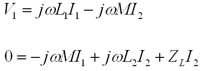
Within the coupled inductor model, these equations are general and apply for arbitrary coupling coefficient k and arbitrary complex load ZL.
Assuming only symmetrically wrapped windings, where N2 and N1 are the winding turns of the secondary L2 and primary L1 inductors respectively, so that the turns ratio N21=N2/N1 is simply related to the primary and secondary inductor values, and
solving the coupled equations above, we obtain the frequency-dependent voltage gain V2/V1 and the effective input impedance Zin for arbitrary coupling k and arbitrary complex load ZL as:

Note that for a given turns ration N21, the voltage gain and input impedance deviate from "ideal" transformer behaviour by factors that depend on the ratio of the load impedance to the secondary inductive
impedance jωL2/ZL.
Limiting Behaviour
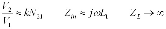
If ZL is very large (e.g. an open output circuit), we obtain exactly as expected:
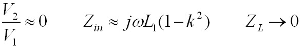
and if ZL is extremely small (e.g. an output short circuit), we obtain:
Perfect Coupling: k=1
For the perfect coupling case with k=1, the voltage gain becomes frequency-independent (but not the effective input impedance) and the equations simplify to:
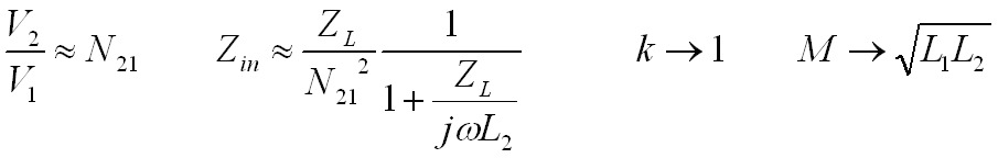
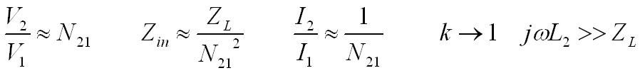
Finally, if the secondary inductive reactance is much greater than the load impedance jωL2 >> ZL, we obtain the familiar ideal transformer results:
Resistive Load: ZL=RL
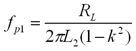
For a pure resistive load, the general gain equation V2/V1 above exhibits a single pole with a (-3dB) corner frequency fp1of:
The frequency rolloff is essentially an "RL" rolloff with the bandwidth increasing as the coupling increases, approaching infinite bandwidth as k->1.
The general input impedance Zin exhibits a zero at DC, a pole at low frequency fp2, and a zero at higher frequency fz. This higher zero frequency
is identical to the pole frequency for the gain :

The zero at DC for Zin means that Zin approaches the inductive impedance jωL1 at very low frequency and will decrease linearly with decreasing f. However, as f->0,
the DC resistance of the transformer primary inductor will eventually dominate and the input impedance will tend to a constant real value.
Example:
The plots below use the exact general expressions above for input impedance and gain within the coupled inductor transformer model with a pure resistive load.
It is important to understand that even with a purely resistive transformer load, and without transformer series resistance and shunt capacitance,
frequency dependent effects are manifested.
Both graphs are
for a nominal 10:1 step down transformer with L1=100H and L2=1H. With an output resistive load impedance of 8 Ω,
the expected "ideal" reflected input impedance is 800 Ω The upper graph shows
the results for a modest coupling coefficient of 0.95 and the lower graph shows a much more "ideal" result for k=0.9999. For k=0.95, fp1= fz = 13Hz while for
k=0.999, fp1= fz = 6.4kHz. For both values of k, fp2 = 1.3Hz. With very high transformer primary
and secondary inductance values as in this example, it is evident that very high values of the coupling coefficient are required to achieve a fairly uniform
effective input impedance for a resistive output load and uniform voltage gain transformation over a wide frequency range:


Transformer Calculator
 The calculator below computes the effective complex input impedance Zin and voltage gain V2/V1 using the general expressions
above for an output load ZL consisting of a series resistor and inductor in parallel with a capacitance as shown in the schematic to the right. This type of load
might represent, for example, a simplified model for a loudspeaker connected to a transformer secondary in an audio amplifier circuit with transformer
output coupling. Zin would correspond to the effective (complex) load impedance in the transistor or tube circuit which will determine the circuit gain.The total
output load impedance ZL of these three components is also displayed. The complex quantities are displayed as magnitude and phase.
This tool provides assistance with quickly determining the deviation that can be expected
for various transformer loads at any frequency for resistive or reactive secondary loads. It also demonstrates various regimes where the coupling
coefficient can have a strong effect on deviation from ideal transformer behaviour.
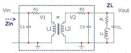
The calculator below computes the effective complex input impedance Zin and voltage gain V2/V1 using the general expressions
above for an output load ZL consisting of a series resistor and inductor in parallel with a capacitance as shown in the schematic to the right. This type of load
might represent, for example, a simplified model for a loudspeaker connected to a transformer secondary in an audio amplifier circuit with transformer
output coupling. Zin would correspond to the effective (complex) load impedance in the transistor or tube circuit which will determine the circuit gain.The total
output load impedance ZL of these three components is also displayed. The complex quantities are displayed as magnitude and phase.
This tool provides assistance with quickly determining the deviation that can be expected
for various transformer loads at any frequency for resistive or reactive secondary loads. It also demonstrates various regimes where the coupling
coefficient can have a strong effect on deviation from ideal transformer behaviour.
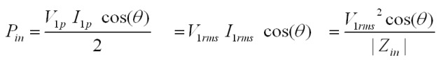
Since the phase angle θ between the input voltage and current is the same, by definition, as the phase angle for the input impedance Zin, the
average power delivered into the primary of the transformer (which must be identical to that dissipated by the resistive part of the load RL) is:
A more accurate model for a transformer as shown below includes transformer series resistances R1, R2 and shunt capacitances C1, C2.
It is easy to extend the model above to include these parameters. R2 and C2 are simply included in a modified total output complex load
impedance ZL to calculate Zin to the right of R1. Then R1, C1 and R2, C2 are included as basic voltage divider networks
before and after the basic gain V2/V1 calculated previously to determine the total overall gain Vout/Vin:
References