
Sommerfeld TM0 Wire Wave
May 24, 2014
It is well known (Stratton 1941, Sommerfeld 1952) that an infinite straight cylindrical homogeneous medium embedded in a homogeneous medium supports an infinity of guided electromagnetic
modes. The various types of modes for different media types have been discussed in detail by these authors. For the case of a typical conducting cylindrical medium embedded
in a medium with low loss, only the lowest order symmetrical TM0 mode or principal mode propogates with relatively low loss compared to all other modes.
Dielectric Constant, Conductivity and Refractive Index
Using the convention for the time factor below and using SI units, the bulk material propogation constant k for a time harmonic plane wave EM field at angular
frequency ω = 2πf, dielectric constant ε and refractive index n for a general medium are all complex:


where the values for the constants vacuum permeability μ0, permittivity ε0 and speed of light c are all exact.
For a lossy medium, the imaginary parts of the material refractive index n and dielectric constant ε/ε0 are positive using the sign convention below.
Depending on the wavelength/frequency being considered, separation
of the material properties into an "inner" complex permittivity εi associated with bound charge and a conductivity σ associated with free charge may be artificial.
At sufficiently high frequency the conductivity σ parameter associated with free charge will become complex due to the finite carrier scattering time compared to the optical period (Ramo 1984).
In any case, the net response of
any homogeneous material to a time harmonic EM field at a specific frequency can always be described by a complex dielectric constant or a complex refractive index.
TM0 Modes
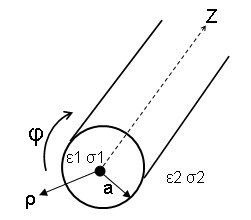
For the axially symmetric TM0 waves, there are three field components Hφ Eρ and Ez ,
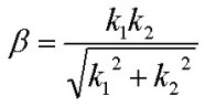
each characterized by a complex modal propogation constant β along the z direction, or equivalently by a complex "mode" refractive index nm.
The functional dependence of each field component is:


where the radial field dependence f(ρ) is different for each field component and involves Bessel function Jo, J1 and Hankel functions Ho1, H11 within and outside
the cylindrical conductor respectively:
Interface matching of tangential E and H fields leads to an exact transcendental equation, for arbitrary material parameters in either region. The solutions of this equation,
for nonmagnetic media, are the propogation constants β describing all axially symmetric TM0 modes (Stratton 1941) :

where u and v are radial propogation constant parameters for f(ρ) evaluated at the wire radius a:

The Principal TM0 Mode
Although the solutions of the exact equation above apply to arbitrary media properties in the wire and external region, for the case of interest here with a good wire conductor and an external dielectric
with low loss, there is only one axially symmetric TM mode solution with fairly low loss. This solution has been called the principal TM wave solution (Sommerfeld) and for this
mode, |k2| ~ |beta|.
In this case, various approximations can be used based on the radial propogation constant parameter values u and v. For any practical conductor diameter, |v| <<1:

and if the wire is a good conductor so that the conduction current is much larger than the displacement current:

For the TM0 principal mode :

and the left hand side of the equation above is a constant, independent of β.
If in addition the wire radius is not too small, the equation above simplies further:

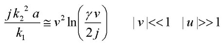
Either equation can be used in a rapidly converting successive approximations iterative algorithm (Sommerfeld) to solve for ξ and therefore v and hence β for the principal TM0 wave solution:

where γ is the constant 1.781072417990197 .. (exponential of Euler constant).
The accuracy of the solutions using this iterative procedure can be easily verified against the exact transcendental equation above by direct substitution.
TM0 Principal TM Wave Calculator
The calculator below uses the Sommerfeld iteration procedure above to accurately compute the TM0 principal wave propogation constant β and propogation loss
for arbitrary dielectric constant and conductivity of both media, provided the approximation |v|<<1 applies and that the wire conductor is a good one so that k1r = k1i.
|u| can have arbitrary value (i.e. the wire radius can be arbitrarily small) and Jo(u)/J1(u) is calculated directly during iteration. Pz is the total axial power flowing along
the wire in the external dielectric, normalized to total conduction current squared in the wire cross section at that z value.
(For any reasonable conductor, the axial
power flow INSIDE the central conductor is extremely small). ρ_75% is a measure of the power extension and is
the radial distance in which approximately 75% of the total power Pz is contained. It is calculated using approximate expressions from Goubau (1950).
Zs is the surface impedance of the center conductor (see below) and δ1 is the skin depth of the center conductor:
Example
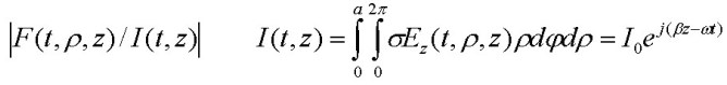
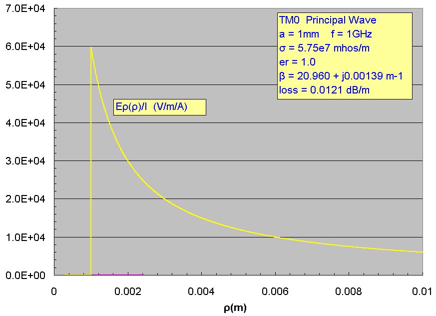
A specific numerical example for the TM principal mode is shown below for a copper wire of radius 1mm in free space at a frequency of 1 GHz. The radial dependence of the magnitude for each field component
is displayed normalized to the total conduction current I integrated through the cross sectional area of the wire (Stratton 1941) where I0 is the total current amplitude
in the wire at z=0 which provides the single arbitrary coefficient for the field amplitudes.
The total cross-sectional current I(t,z) contains the temporal and z dependence:
The alternating-current complex impedance (Stratton 1941) or surface impedance Zs in Ω/m is defined as the ratio of the axial electric field at the surface of
the conductor to the total conduction current, integrated over the wire cross-section, at the same time and axial position (t,z). This is the internal impedance of the center conductor
and does not include the "external" impedance due to magnetic field generated outside the center conductor:

At high frequency, the real and imaginary parts of the surface impedance are nearly identical, with the imaginary part being inductive. This means that at high frequency,
the surface axial electric field and the total conduction current are out of phase my 45 degrees (as are Ez and Hphi at the surface of the wire). For a detailed discussion of
the frequency dependence of Zs see Coaxial Cable ....
At 1 GHz (λ0 = 300mm) the skin depth for copper is very small at ~ 2 µm and although the Ez and Hφ field components
are continuous across the interface, all field components drop extremely rapidly as shown.
Although the axial electric field Ez(rho) outside the wire is weak compared to the radial component,
it extends out further:


The time-averaged Poynting vectors (power flow) for the axial z component Sz(ρ, z)and outward directed ρ component Sρ(ρ, z) are:
and are displayed below normalized to the total current squared (in units of Ω/m^2). The radial component of power flow is directed INWARD (negative). For a typical good conductor,
all the axial power flow is carried outside the wire. The inward radial flow of power enters the wire and is rapidly attenuated as dissipation in the wire conductor:

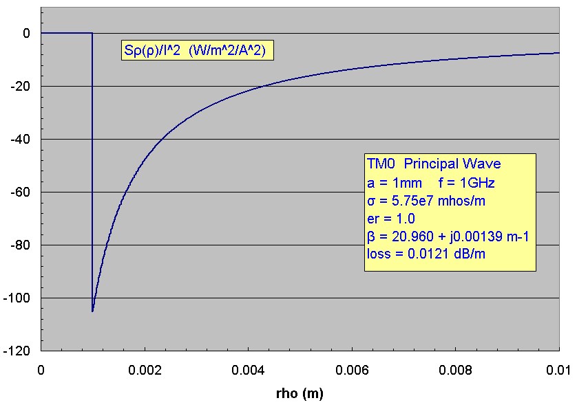
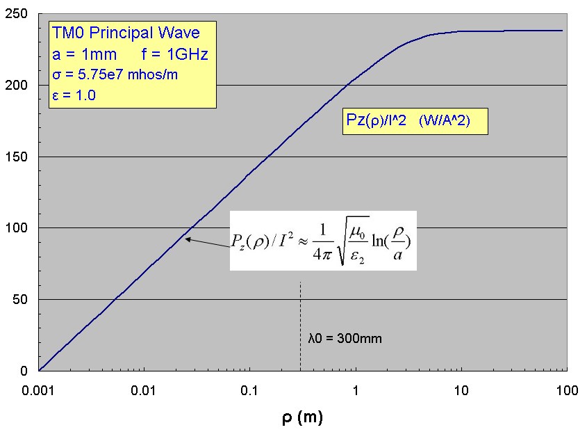
Although the power density Sz(ρ) outside the wire appears to be confined near the wire,
in fact only 50% of the total axial power flow in the principal mode is contained in a radius of 50 mm, 75% in a radius of 390 mm and 90% within a radius of 1.4m.
The power Pz(ρ) flowing in the z direction within a radius ρ is obtained by integrated Sz radially over a circular area. Extending the range to infinity
gives the finite total power:
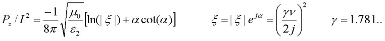
where ξ and therefore ν are solutions of the transcendental equation above for the TM wire wave mode.
For the example here Pz /I^2 ~ 237.4 W/A^2 as shown in the cumulative axial power flow plot below. The results computed
here, which are accurate over the entire range of ρ, agree closely with approximate graphical results presented by Goubau (1950).
Since |v| << 1 for a typical TM0 principal wave, the fields Hφ and Eρ, which have a H11 dependence, decrease nearly as 1/ρ so the integrated power
in a circular area of radius ρ will increase logarithmically as shown and the axially power flowing outside the wire can be easily computed using Ampere's law for the magnetic
field with total conduction current in the cylindrical conductor and by noting that the radial electric field is related exactly as for a plane wave (assuming the external medium is a good dielectric
with very low conductivity). Eventually however for sufficiently large ρ the H11 dependence will become exponential
which causes Sz to drop more quickly and hence the total power to approach a fixed value. This transition will occur at a radial distance such that |v|ρ/a ~ 1.
The axial flow of power WITHIN the conductor is completely negligible for any realistic conductor, so all the propogated power of the wire wave is carried external to the central conductor:
The propogation loss of the TM mode is described by βim. Inward power flow to the conductor (per unit length) from the external dielectric is the source
of the mode attenuation. In terms of power loss:

For the example above, the total axial power is 238 W/A^2 and the inward radial average power density Sρ(ρ=a) is 105 W/m^2/A^2. The loss
expression leads to βim = 0.00139 m-1 in agreement with the β mode calculation for this example.
Limit of Large Wire Radius
For very large wire radius, |v| >1 and the approximation used in the iterative procedure above is invalid. In this limit, the exact transcendental equation above should approach
the result for the surface wave
for a planar interface. In this limit both |v| >>1 and |u| >>1 and ratio of Bessel and Hankel functions become:
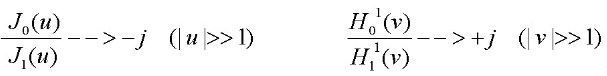
leading to the simple result for the planar TM0 surface wave:
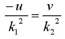
and substituting for u and v, the following elegant symmetric expression is obtained for the propogation contant of the TM0 mode for an ideal infinite planar interface, in agreement with
the result obtained from direct analysis of the planar case:
For the example above with copper at 1GHz, the planar interface propogation loss result is 8.8e-8 dB/m, much lower than the result for the wire propogation loss.
Reference:
- Electromagnetic Theory, J. Stratton, 1941, McGraw Hill, pp. 524-536
- Electrodynamics, A. Sommerfeld, Lectures on Theoretical Physics, 1952, VIII Academic Press, pp 177-185
- Surface Waves and Their Application to Transmission Lines, G. Goubau, J. Appl. Phys, V21, 1950, p.1119
- Field Theory of Guided Waves, R. E. Collin, 1991, IEEE Press, pp.697-700
- Fields and Waves in Communication Electronics, S. Ramo, J. Whinnery, T. Van Duzer, 1984, J. Wiley & Sons. pp. 279-283